Code
import numpy as np
from sklearn.datasets import load_svmlight_file
import matplotlib.pyplot as plt
We will learn the basics of applying logistic regression and support vector machines (SVMs) to classification problems. You’ll use the scikit-learn library to fit classification models to real data.
This Applying logistic regression and SVM is part of Datacamp course: Linear Classifiers in Python
This is my learning experience of data science through DataCamp
import numpy as np
from sklearn.datasets import load_svmlight_file
import matplotlib.pyplot as pltWe will explore subset of Large movie review dataset The X variables contain features based on the words in the movie reviews, and the y variables contain labels for whether the review sentiment is positive (+1) or negative (-1).
X_train, y_train = load_svmlight_file('dataset/aclImdb_v1/aclImdb/train/labeledBow.feat')
X_test, y_test = load_svmlight_file('dataset/aclImdb_v1/aclImdb/test/labeledBow.feat')X_train.shape(1347, 64)X_test.shape(450, 64)type(X_train)numpy.ndarrayX_train[0]array([ 0., 0., 0., 3., 16., 3., 0., 0., 0., 0., 0., 12., 16.,
2., 0., 0., 0., 0., 8., 16., 16., 4., 0., 0., 0., 7.,
16., 15., 16., 12., 11., 0., 0., 8., 16., 16., 16., 13., 3.,
0., 0., 0., 0., 7., 14., 1., 0., 0., 0., 0., 0., 6.,
16., 0., 0., 0., 0., 0., 0., 4., 14., 0., 0., 0.])y_train[y_train < 5] = -1.0
y_train[y_train >=5] = 1.0
y_test[y_test < 5] = -1.0
y_test[y_test >= 5] = 1.0from sklearn.neighbors import KNeighborsClassifier
# Create and fit the model
knn = KNeighborsClassifier()
knn.fit(X_train[:, :89523], y_train)
# Predict on the test features, print the results
pred = knn.predict(X_test)[0]
print("Prediction for test example 0:", pred)Prediction for test example 0: 1.0In this exercise, you’ll apply logistic regression and a support vector machine to classify images of handwritten digits.
from sklearn import datasets
from sklearn.model_selection import train_test_split
from sklearn.linear_model import LogisticRegression
from sklearn.svm import SVC

digits = datasets.load_digits()
X_train, X_test, y_train, y_test = train_test_split(digits.data, digits.target)

# Apply logistic regression and print scores
lr = LogisticRegression()
lr.fit(X_train, y_train)
print(lr.score(X_train, y_train))
print(lr.score(X_test, y_test))
1.0
0.9622222222222222C:\Users\dghr201\AppData\Local\Programs\Python\Python39\lib\site-packages\sklearn\linear_model\_logistic.py:444: ConvergenceWarning: lbfgs failed to converge (status=1):
STOP: TOTAL NO. of ITERATIONS REACHED LIMIT.
Increase the number of iterations (max_iter) or scale the data as shown in:
https://scikit-learn.org/stable/modules/preprocessing.html
Please also refer to the documentation for alternative solver options:
https://scikit-learn.org/stable/modules/linear_model.html#logistic-regression
n_iter_i = _check_optimize_result(# Apply SVM and print scores
svm = SVC()
svm.fit(X_train, y_train)
print(svm.score(X_train, y_train))
print(svm.score(X_test, y_test))0.994060876020787
0.9911111111111112In this exercise you’ll explore the probabilities outputted by logistic regression on a subset of the Large Movie Review Dataset.
The variables X and y are already loaded into the environment. X contains features based on the number of times words appear in the movie reviews, and y contains labels for whether the review sentiment is positive (+1) or negative (-1).
# Instantiate logistic regression and train
lr = LogisticRegression()
lr.fit(X, y)

# Predict sentiment for a glowing review
review1 = "LOVED IT! This movie was amazing. Top 10 this year."
review1_features = get_features(review1)
print("Review:", review1)
print("Probability of positive review:", lr.predict_proba(review1_features)[0,1])
# Review: LOVED IT! This movie was amazing. Top 10 this year.
# Probability of positive review: 0.8079007873616059


# Predict sentiment for a poor review
review2 = "Total junk! I'll never watch a film by that director again, no matter how good the reviews."
review2_features = get_features(review2)
print("Review:", review2)
print("Probability of positive review:", lr.predict_proba(review2_features)[0,1])

# Review: Total junk! I'll never watch a film by that director again, no matter how good the reviews.
# Probability of positive review: 0.5855117402793947def make_meshgrid(x, y, h=.02, lims=None):
"""Create a mesh of points to plot in
Parameters
----------
x: data to base x-axis meshgrid on
y: data to base y-axis meshgrid on
h: stepsize for meshgrid, optional
Returns
-------
xx, yy : ndarray
"""
if lims is None:
x_min, x_max = x.min() - 1, x.max() + 1
y_min, y_max = y.min() - 1, y.max() + 1
else:
x_min, x_max, y_min, y_max = lims
xx, yy = np.meshgrid(np.arange(x_min, x_max, h),
np.arange(y_min, y_max, h))
return xx, yydef plot_contours(ax, clf, xx, yy, proba=False, **params):
"""Plot the decision boundaries for a classifier.
Parameters
----------
ax: matplotlib axes object
clf: a classifier
xx: meshgrid ndarray
yy: meshgrid ndarray
params: dictionary of params to pass to contourf, optional
"""
if proba:
Z = clf.predict_proba(np.c_[xx.ravel(), yy.ravel()])[:,-1]
Z = Z.reshape(xx.shape)
out = ax.imshow(Z,extent=(np.min(xx), np.max(xx), np.min(yy), np.max(yy)),
origin='lower', vmin=0, vmax=1, **params)
ax.contour(xx, yy, Z, levels=[0.5])
else:
Z = clf.predict(np.c_[xx.ravel(), yy.ravel()])
Z = Z.reshape(xx.shape)
out = ax.contourf(xx, yy, Z, **params)
return outdef plot_classifier(X, y, clf, ax=None, ticks=False, proba=False, lims=None):
# assumes classifier "clf" is already fit
X0, X1 = X[:, 0], X[:, 1]
xx, yy = make_meshgrid(X0, X1, lims=lims)
if ax is None:
plt.figure()
ax = plt.gca()
show = True
else:
show = False
# can abstract some of this into a higher-level function for learners to call
cs = plot_contours(ax, clf, xx, yy, cmap=plt.cm.coolwarm, alpha=0.8, proba=proba)
if proba:
cbar = plt.colorbar(cs)
cbar.ax.set_ylabel('probability of red $\Delta$ class', fontsize=20, rotation=270, labelpad=30)
cbar.ax.tick_params(labelsize=14)
#ax.scatter(X0, X1, c=y, cmap=plt.cm.coolwarm, s=30, edgecolors=\'k\', linewidth=1)
labels = np.unique(y)
if len(labels) == 2:
ax.scatter(X0[y==labels[0]], X1[y==labels[0]], cmap=plt.cm.coolwarm,
s=60, c='b', marker='o', edgecolors='k')
ax.scatter(X0[y==labels[1]], X1[y==labels[1]], cmap=plt.cm.coolwarm,
s=60, c='r', marker='^', edgecolors='k')
else:
ax.scatter(X0, X1, c=y, cmap=plt.cm.coolwarm, s=50, edgecolors='k', linewidth=1)
ax.set_xlim(xx.min(), xx.max())
ax.set_ylim(yy.min(), yy.max())
# ax.set_xlabel(data.feature_names[0])
# ax.set_ylabel(data.feature_names[1])
if ticks:
ax.set_xticks(())
ax.set_yticks(())
# ax.set_title(title)
if show:
plt.show()
else:
return axdef plot_4_classifiers(X, y, clfs):
# Set-up 2x2 grid for plotting.
fig, sub = plt.subplots(2, 2)
plt.subplots_adjust(wspace=0.2, hspace=0.2)
for clf, ax, title in zip(clfs, sub.flatten(), ("(1)", "(2)", "(3)", "(4)")):
# clf.fit(X, y)
plot_classifier(X, y, clf, ax, ticks=True)
ax.set_title(title)#hide
X = np.array([[11.45, 2.4 ],
[13.62, 4.95],
[13.88, 1.89],
[12.42, 2.55],
[12.81, 2.31],
[12.58, 1.29],
[13.83, 1.57],
[13.07, 1.5 ],
[12.7 , 3.55],
[13.77, 1.9 ],
[12.84, 2.96],
[12.37, 1.63],
[13.51, 1.8 ],
[13.87, 1.9 ],
[12.08, 1.39],
[13.58, 1.66],
[13.08, 3.9 ],
[11.79, 2.13],
[12.45, 3.03],
[13.68, 1.83],
[13.52, 3.17],
[13.5 , 3.12],
[12.87, 4.61],
[14.02, 1.68],
[12.29, 3.17],
[12.08, 1.13],
[12.7 , 3.87],
[11.03, 1.51],
[13.32, 3.24],
[14.13, 4.1 ],
[13.49, 1.66],
[11.84, 2.89],
[13.05, 2.05],
[12.72, 1.81],
[12.82, 3.37],
[13.4 , 4.6 ],
[14.22, 3.99],
[13.72, 1.43],
[12.93, 2.81],
[11.64, 2.06],
[12.29, 1.61],
[11.65, 1.67],
[13.28, 1.64],
[12.93, 3.8 ],
[13.86, 1.35],
[11.82, 1.72],
[12.37, 1.17],
[12.42, 1.61],
[13.9 , 1.68],
[14.16, 2.51]])
y = np.array([ True, True, False, True, True, True, False, False, True,
False, True, True, False, False, True, False, True, True,
True, False, True, True, True, False, True, True, True,
True, True, True, True, True, False, True, True, True,
False, False, True, True, True, True, False, False, False,
True, True, True, False, True])from sklearn.svm import LinearSVC
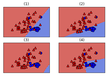
# Define the classifiers
classifiers = [LogisticRegression(), LinearSVC(), SVC(), KNeighborsClassifier()]
# Fit the classifiers
for c in classifiers:
c.fit(X, y)
# Plot the classifiers
plot_4_classifiers(X, y, classifiers)C:\Users\dghr201\AppData\Local\Programs\Python\Python39\lib\site-packages\sklearn\svm\_base.py:1225: ConvergenceWarning: Liblinear failed to converge, increase the number of iterations.
warnings.warn(